|
Abstract: The Watershed Planning System (WPS) is a geographic-based decision support system designed to help local governments and State agencies developed coordinated land and non-point source pollution management strategies. It enhances our ability to provide a systematic, comprehensive evaluation of non-point source pollution and land use issues that reflect realistic watershed conditions and management alternatives. The output provides a basis for selecting feasible mix of management alternatives that can be implemented through program changes (such as: comprehensive plans, soil conservation and water quality plans, nutrient management programs, zoning and subdivision programs and sensitive area protection programs, etc.) and through BMP implementation.
INTRODUCTION
The Maryland Department of Planning (MDP) has developed the Watershed Planning System (WPS) to provide sound technical and programmatic multi-scale decision-support for coordinated management of new growth, land use, natural resources, and non point source pollution. Watershed Planning System is a GIS-based land use model designed to assess and identify growth management alternatives that will minimize impacts on land and water resources at the county, subcatchment, and tributary scale. The data used (land use, county zoning and sewer service, environmental regulations, transportation analysis zones, census data and physiographic characteristic) in the models are customized to each county. Therefore, the model results can be easily used by the other state agencies, counties, and local jurisdictions. It uses the change in development patterns, loss of resource land, forested buffers, and corresponding changes in nutrient loads to evaluate different land use and management scenarios.
Watershed Planning System Overview
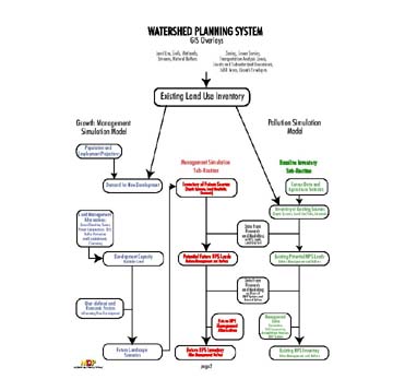
The WPS consists of two computer models: Pollution Simulation Model and the Growth Management Simulation Model (Figure 1). The Pollution Simulation Model is designed to estimate the relative nutrient loads from on-site disposal systems, various categories of land use/land cover, and areas of concentrated animal populations and exposed waste storage facilities. The Growth Management Simulation Model estimates the change in land uses and sensitive areas by subcatchment as a function of population and household projections. The model allows evaluation of different future land use scenarios by changing assumptions associated with comprehensive plans and the zoning, subdivision, and environmental regulations.
The models use data from composite geographic information system (GIS) overlays. GIS coverages include, for each county:
- Current land use / land cover (Table 1), preserved (State, Federal, County, and private conservation ownership or easements) lands, soils, streams and waterways, political boundaries, zoning, sewer service plans, transportation analysis zones, and growth boundaries.
- Enhanced parcel data base derived from Maryland Property View.
Table I : Maryland Office of Planning Land Use Categories
| I I |
Low Density Residential |
90% or More Single Family/Duplex Dwellings |
0.2 to 2.0 |
| 12 |
Moderate Density Residential |
90% or More Single Family/Duplex Dwellings Or Attached Single-Unit Row Houses |
2.0 to 8.0 |
| 13 |
High Density Residential |
90% Or More Attached Single-Unit Row House Garden Apartments, High Rise Apartment/ Condominiums, Mobile Home & Trailer Park |
8 or more |
| 14 |
Commercial |
Retail & Wholesale |
N/A |
| 15 |
Industrial |
Manufacturing & Industrial Parks |
N/A |
| 16 |
Institutional |
Schools, Military Installation (Build-out only) Church, Medical facilities & Correctional Institutions |
N/A |
| 17 |
Extractive |
Surface Mining |
N/A |
| 18 |
Open Urban Land |
Urban Areas Whose Use Does Not Require Structures (Golf Courses, Parks) |
N/A |
| 191 |
Large Lot Agricultural |
Dominant Land Cover Open Field or Pasture |
0.2 to 0.05 |
| 192 |
Large Lot Forest |
Dominant Land Cover Forest |
0.2 to 0.05 |
| 21 |
Cropland |
Field Crops & Forage Crops |
N/A |
| 22 |
Pasture |
Permanent and Rotated |
N/A |
| 23 |
Orchards/Vineyard s/ Horticulture |
Intensively Managed Commercial Bush & Tree Crops |
N/A |
| 24 |
Feeding Operations |
Feed lots & Poultry Houses |
N/A |
| 25 |
Row & Garden Crops |
Truck & Vegetable Farms |
N/A |
| 40 |
Forest |
Forest and Brush |
N/A |
| 242 |
Agricultural Buildings |
Storage Facilities, Build Out Associated With A Farmstead |
N/A |
| 241 |
Feeding Operations |
Feedlots, Holding Lots for Animals, and Exposed Waste Storage Facilities |
N/A |
| 60 |
Wetland |
Rivers, Waterways, Reservoirs, Bays Estuaries, Ponds, and Oceans |
N/A |
| 70 |
Bare Ground |
Areas of Exposed Ground Caused Naturally by Construction or by Other Cultural Processes |
N/A |
The GIS files are linked, through common fields or variables, to other files to provide information on specific allowances / requirements of land use and conservation plans and programs of local government. Each model combines the basic landscape data with additional watershed information, such as census data and management practices, compiled in cooperation with State and local governments.
The key utility of the WPS as a planning tool is its ability to readily represent realistic alternatives in terms of management programs. The approach can be applied in any part of the State. The smallest unit of analysis is the subcatchment scale allowing results to be aggregated to the county, watershed, and/or tributary scale. The models use standardized GIS layers to characterize important landscape features and represent planning and management boundaries. These, however, are customized where more accurate data or data of finer resolution exists. The limits, requirements, and constraints of State and local plans, programs, and regulations are used in the models to determine the potential for development and conservation of resource land and sensitive areas in each subwatershed. By following coordination procedures with local jurisdictions and State and local programs, the alternatives evaluated through the models represent feasible program and BMP options.
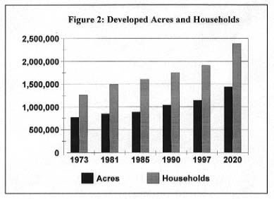
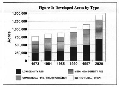
The system is designed to easily incorporate data from ongoing NPS research and modeling, allowing updating and refinement, and to represent a range of plans and management strategies. To date, the WPS has been applied in the seven counties (Anne Arundel, Calvert, Charles, Howard, Montgomery, Prince George's and St. Mary's counties) that comprise the Lower Potomac, Lower Western Shore and the Patuxent Tributaries, and Worcester and Harford Counties, to address a variety of land use management, resource conservation, and pollution control objectives. In addition, the model has been used to produce statewide 2020 land use projections (Figure 2 and 3).
Pollution Simulation Model
The Pollution Simulation Model is designed to estimate the relative nutrient loads from on-site disposal systems, various categories of land use/land cover, and areas of concentrated animal populations and exposed waste storage facilities. It is composed of two subroutines - The Baseline Inventory and the Management Simulation. The Baseline Inventory provides an inventory of existing land use conditions and nonpoint source management practices, with respect to nutrient loads generated from the landscape by specific categories. The Management Simulation sub-routine estimates the potential impacts non-point source management alternatives on pollution loads. This is used to evaluate the effects of NPS management alternatives on current land use conditions and potential future land use conditions. When used in the latter capacity, the potential effects of alternative planning, zoning, and subdivision regulations on NPS loads are also evaluated.
The loading estimates for each source are partitioned among three flow pathways: surface runoff, shallow subsurface flow, and deeper groundwater flow (OP, 1994: OP, 1995). Partitioning factors are derived from Chesapeake Bay Program Office's Watershed Model by segment (MDE, 1993; Lewis Linker, Personal Communication). This important feature of the WPS facilitates a more realistic evaluation of the effects of management practices, which affect loads moving through different pathways in different ways. Thus, a county proposing to use different stormwater management practices can examine the effects on pollution for different planning and zoning schemes (such as, traditional versus clustering land use patterns). The effects of urban nutrient control alternatives can be reviewed in relation to different land use patterns and other non-point source controls, such as agricultural controls or pollution buffers. The result is a relatively comprehensive context for watershed planning and decision making.
The model estimates the nutrient loads generated from the current landscape by source category (land use/soil combination). The landscape is divided into source categories based on MDP's land use and soils (OP, 1973). The Maryland Natural Soil Groups were rated for their potential to export nitrogen and phosphorus with assistance from NRCS. Data compiled from non-point source management programs, research, monitoring, and models are compiled and used to set the input parameters for estimating the Baseline Inventory (OP, 1993; OP, 1994). For each source category the Baseline Inventory estimates the relative pollution load by land use; the effects of existing management systems and pollution buffers (forest and wetlands); and the total loads generated from the subcatchment to surface waters (edge of stream load). Chesapeake Bay Program Watershed Model delivery factors are used to estimate the amount of nitrogen or phosphorus that reaches the Bay.
Growth Management Simulation Model
The Growth Management Simulation model projects the existing land inventory into a series of possible "future" landscapes, each a function of different land use management alternatives. Land use changes and the loss or gain of pollution buffers depend on the individual county plans, regulations, and management procedures simulated.
Changes in land uses and environmentally sensitive areas are estimated using population projections and growth management factors as independent variables. The model evaluates different possible land use scenarios by changing assumptions about comprehensive plans, zoning plans, sewer service, subdivision and environmental regulations. New development is then calculated as a function of household demand, existing or hypothetical management choices (such as, clustering, transfer of development rights, growth areas, and agricultural land preservation) and user-defined considerations. User-defined considerations allow local concerns, and policies that may influence the type and locations of development to be represented in the
GIS input into the model includes an improved MdPropertyView point database, and polygon frequency file of a composite GIS intersections. This composite coverage includes 1997 land use, zoning, protected lands, sewer service, watersheds, and priority funding areas. The improved parcel point database been tagged with attributes with the GIS coverages mentioned above, and checked for accuracy in the acres field. This check was performed using a program to scan through the legal descriptions and correct any anomalies in the acres field against the legal field. Secondly, parcels with extremely large acres were compared to the parcel maps to corroborate their actual size.
The growth portion of the WPS is broken in two main components for our purposes, the MdPropertyView point analysis and the land use polygon calculations. Point analysis is where the we calculate capacity, development probability, and future change in land use driven by demand and capacity. Once this is complete, the demand for new development is then summarized by development type and combined with the base 1997 land use to give us our final 2020 land use projections.
The development capacity for each parcel in the State is calculated based on subdivision regulations, zoning and sewer service. This information has been compiled for the 23 Counties over the last year both from a survey sent to each County, phone conversations to clarify details and reading of subdivision regulations, septic health regulations, and zoning ordinances. Also taken into account are the critical area (if available), County, State and Federal protected lands, existing development, and the potential for infill. Under normal zoning conditions, the residential development capacity is equal to the lot size multiplied by the realized density (based on the average lot yields provided by the county). This may be adjusted to account for nuances of clustering, infill and County specific protective zones. The demand is based on the Round VI Small Area Forecasts for Transportation Analysis Zone if available. Otherwise, the model partitions MDP new household projections by subwatershed based on historical development patterns over the last five years (1992-97). Demand for each subwatershed is then allocated to parcels with capacity located within each specific subwatershed.
Non-residential development is driven by the MDP's projections of employment jobs by place of work. The underlying assumption is the ratios of acreage of employment land uses to the number of employees remains constant form 1997 to 2020. Based on this assumption, as employment grows, commercial, and industrial land acreage grow correspondingly. The demand for employment acreage is then apportioned to appropriately zoned land. The demand for new development has now been calculated. The next step is to summarize this demand from the parcel level and allocate it to the existing land use/land cover. The demand is summarized to a zoning-watershed unit of analysis and apportioned out the to the polygons in the corresponding unit of analysis. Extra demand is sent to surrounding units of analysis if demand exceeds the amount of developable land. Infill development is converted from the appropriate land use; low- moderate, or high density residential, and new development is apportioned to forest and agriculture proportionately to the amount of developable land in each land use present in each unit of analysis.
References
Maryland Department of Environment (1993) Chesapeake Bay HSPF Model - Patuxent River.
Memorandum: Final agricultural BMP reduction efficiencies. Dr. William Majette, August 1994
Nonpoint Source Subcommittee On-Site System Workshop Conference (1992) Findings and Recommendations
Maryland Office of Planning, (1973). Natural soil Groups Technical Report, Baltimore, MD.
Maryland Office of Planning (1993) Nonpoint Source Assessment and Accounting System: Final Report for FFY'91 Section 319 Grant Baltimore, Maryland.
Maryland Office of Planning (1994 Patuxent Watershed Demonstration Project: Phase I Interim Guidance Document Baltimore, Maryland.
Maryland Office of Planning (1995). Development and Application of the Nonpoint Source Assessment and Accounting System Final Report for FFY'92 Section 319 Grant Baltimore, Maryland.
Personnel Communication: Partitioning of Nutrient Loads to Surface, Subsurface and Groundwater Pathways. Lewis Linker, Chesapeake Bay Program, 1994.
Personnel Communication: Rating of NSGs for their Potential to Export N and P. James Brown, State Soil Conservation Service. 1992.
Author and Copyright Information
Copyright 2001 by Authors
|