|
INTRODUCTION
Grand Traverse Bay and the Grand Traverse Bay Watershed (GTBW) are important natural and economic resources for Michigan and the Great Lakes Region, due to their great scenic beauty, quality of waters, and the recreational opportunities these afford. However, the watershed is currently undergoing some of the most rapid population growth and land-use change of any region in the Great Lakes States (Vesterby and Heimlich, 1991). The GTBW Initiative, a not-for-profit organization that works with community groups and university researchers, has identified the following issues of concern in this watershed: erosion and sedimentation, phosphorous and nitrogen inputs to the Bay, degradation of water quality as indicated by algae growth and oxygen depletion in deep waters of the Bay, inputs of toxic substances, and the impact of various land uses and land use protection measures on these (GTBW Initiative Water Quality Monitoring Program Draft, October 16, 1995).
Numerous field studies have demonstrated that changes in land use affect groundwater and surface water dynamics. Potential environmental impacts include 1) the redistribution of recharge and discharge areas, and reduced groundwater discharge to streams (Doe et al, 1996); 2) changes in groundwater recharge rates (Thorburn et. al., 1991); and 3) changes in stream flow and temperature with subsequent influences on stream ecology (Wiley et al. 1997). Likewise, land use/cover patterns and changes in land use/cover have been found to influence surface water chemistry. Effects have also been shown on the chemistry of major ions (Cl) and nutrients (N and P) (Herlihy et al., 1998; Field et al., 1996; Flintrop et al., 1996). Variations in land use change affect surface and groundwater hydrodynamics by varying the amounts of impervious or erodable surfaces and by redirecting water flow paths. Such parameters are often incorporated into models that examine the input of non-point source (NPS) pollutants to surface waters (e.g., N- Skop and and Sorensen, 1998; P- Scott et al. 1998; fecal coliform bacteria – Hunter et al.,1992; Weiskel et al.,1996; and Fraser et al.,1998; groundwater leaching of NPS contaminants – reviewed by Corwin and Wagenet, 1996). These studies underscore the need to quantify the effects of land use on ground water quality and hydrologic dynamics. Spatial-temporal models coupled to geographic information systems (GIS) can be powerful tools to quantify these relationships.
This paper presents the application of one land and two hydrologic models to understand the coupling of land use and water quality in Michigan’s Grand Traverse Bay Watershed. The Land Transformation Model (Pijanowski et al., 1996, Pijanowski et al., 2000a, Pijanowski et al., 2000b) couples Artificial Neural Network (ANN) routines to GIS databases containing information on population growth, transportation factors, and locations of important landscape features such as rivers, lakes, recreational sites, and high-quality vantage points to forecast future land use patterns. The model (Pijanowski et al., 2000a) couples GIS and ANN routines. Details of the LTM simulation presented here can be found in Pijanowski et al. (in press).
The two hydrogeologic models that are being used here allow us to explore the dynamics of groundwater flow paths throughout the GTBW. The first is a two-layer, high-resolution finite-difference groundwater flow model based on the USGS groundwater flow code, MODFLOW. The second is a solute transport model based on MT3D. This solute transport model is being used to quantify the impacts on water quality scenarios (e.g., influence of road salt) to assess potential impacts of individual land uses on water quality. Details of the parameterization of these two models can be found in Boutt et al., 2001. Both models are contained in the Groundwater Modeling System (GMS) graphical user interface, which also reads and writes GIS files.
BACKGROUND
Land Transformation Model
Artificial Neural Networks (ANN) are designed to emulate the functionality of biological neurons in order to achieve a higher parallel processing potential for digital data. ANNs are a branch of information science that are classified as "machine learning algorithms". ANNs differ from other machine learning approaches (e.g., genetic algorithms, cellular automata) in that software mimics how neurons communicate and process information.
There are many different types of ANNs. The multi-layer perceptron (MLP) neural net described by Rumelhart et al. (1986) is one of the most widely used ANNs. The MLP consists of three different types of layers: input, hidden, and output (Figure 1). The MLP allows computers to develop the best possible fit between an input vector (i.e., a series of values associated with the input) and an output value, oftentimes referred to as a "target". ANN algorithms calculate weights for input values, input layer nodes, hidden layer nodes and output layer nodes by introducing the input in a feed forward manner. ANN software is designed to propagate values for weights through a hidden layer or layers and then on to the output layer. The values are then modified according to a set of rules that attempt to minimize the error that fits an expected output value and the actual output value of the dataset.
Artificial Neural Networks have been used in aviation, biomedical, electrical engineering, remote sensing and the social sciences to model complex systems that have not been adequately described through standard state equations.
The neural network based LTM is similar in structure to many regression-type land use change models (Pijanowski et al., in press) that model the relationship between potential drivers (dependent variables) and occurrence of transitions (independent variable). Neural networks, on the other hand, differ significantly from regression-based models in that ANNs use a machine learning approach to develop an numerical solution to fit input (drivers) and output (occurrence or non-occurrence of transitions). Neural networks are: 1) capable of finding nonlinear solutions to fit input and output data, 2) tolerant of errors in data which may be characteristic of classified land use/cover data derived from satellite data, and are 3) capable of generalizing results from one location to another (Skapura, 1996; Swingler, 1996). In the latter instance, generalization means that the neural network can produce a robust model using input data that it has not seen before (as long as the parameterization of the inputs and outputs is the same). Tests of the ability of the ANN-based LTM to generalize across locations have been successful. For example, a neural net model that learned (trained) on data presented for urbanization in the Detroit Metropolitan Area (DMA) and then applied to the Twin Cities Metropolitan Area (TCMA) performed as well as a neural net trained in DMA and tested using a subset of the DMA data (Pijanowski et al., 2001).
The LTM currently employs a multiplayer perceptron (MLP) neural net topology with one or two hidden layers; each layer has at least the same number of nodes as the number of input vectors. Inputs are derived from raster spatial layers; input values are normalized between 0.-1. by dividing by the maximum value in each data layer. Output is composed of locations that transitioned (coded as a 1) and those that did not transition/change (coded as a 0).
METHODS
Study Sites
Michigan's Grand Traverse Bay Watershed (GTBW) is located in the northwestern portion of Michigan’s Lower Peninsula (Figure 2) and is among regions in the United States with the most rapid population growth and land use change (Vesterby and Heimlich, 1991). We extend our land use change modeling exercise to the entire six county region and our groundwater modeling exercise to the area within these six counties that contains the largest watershed. The six counties include: Grand Traverse, Kalkaska, Antrim, Leelanau, Charlevoix and Benzie. From 1970 to 1997, resident population in the watershed nearly doubled. Traverse City is the largest city in the watershed, with a resident population of approximately 18,000 and a tourist population that can exceed 500,000. Land use in the GTBW is predominantly forest (49%) and agriculture (20%). Much of the forested portions of this watershed are managed within the Pere Marquette State Forest, which encompasses most of the upland reaches of the Boardman River tributaries (Figure 2). Urban land use comprises about 6% of the total area of the watershed. The other main land covers are open herbaceous/shrub/grasslands (15%), water (9%), and wetlands (1%).
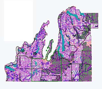
Figure 2. The five county study area that bounds the Grand Traverse Bay Watershed.
Shown are transportation, surface water and the location of major features
(Old Mission Peninsula and Traverse City).
The land use database in this project was obtained through MiRIS (Michigan Resource Information System), which is a statewide database developed around 1980 from 1:24,000 aerial photography. Land uses are classified using a slightly modified version of the Anderson land use / land cover classification system (Anderson et al., 1976). The land use/land cover layer for Grand Traverse County was updated in 1990. This updated layer was obtained from the county’s Drain Commissioner’s Office. For use in this project, all land use codes were reclassified to Anderson Level I land uses. Level I land uses are classified as urban, agriculture, nonforested vegetation (including grasslands, shrubs, herbaceous), deciduous forest, coniferous forest, wetland, open water and barren. Both land use files were then rasterized at a resolution of 100 x 100 meters.
MiRIS line files, digitized from 1:24,000 scale topographic maps, were integrated with our database to represent the transportation network and locations of rivers, lakes, and the Grand Traverse Bay shoreline and provide the appropriate inputs to the GIS-based LTM. USGS digital elevation models (DEM), corresponding to the 7.5-minute topographic quandrangles covering the watershed, were obtained then mosaiced for seamless coverage. DEM data were then resampled to 100 x 100 meter cell sizes. Boundaries for public lands were digitized from county digital DRG databases. Locations of recreational sites, such as golf courses, casinos, ski lodges, and marinas were obtained from published county road maps and stored as point coverages in our GIS. A separate updated MiRIS for Grand Traverse County, representing 1990 land use, was obtained from the County Drain Commissioner’s Office.
LTM Parameterization
Several driving variables were used in the LTM, drawing from several different areas. These driving variable grids are shown in Figure 2; the method of calculating them is summarized below:
Transportation. The Euclidean distance from each cell in the region to the nearest highway and county road was stored in separate Arc/INFO GRID coverages. These two driving variable grids represent the potential accessibility of a location for new development. A third transportation coverage, density of residential streets within a 5 km square window, was created to represent the preponderance of an area to possess residential urban services (e.g., sewers, electricity, cable services) that could make it likely that more residential development could occur in the future.
Landscape Features. The distance from lakes and rivers was also calculated. Pijanowski et al. (in press) has found that landscape topography is an influential factor contributing toward residential use. Thus, a "rolling hills" driving variable grid was created from the 30m Digital Elevation Model (DEM). The amount of topographic variation surrounding each cell was estimated by calculating the standard deviation of all cell elevations within a 5 km square area. Cells containing larger values reflect landscapes that contain a greater amount of topographic relief around them.
Urban Services. The distance each cell was from the nearest urban cell during the start the model was calculated and stored as a separate driving variable grids. It is assumed that the costs of connecting to current urban services (e.g., sewers) decrease with distance from urban.
Exclusionary Zones. In the GTBW, the following areas were held back as being areas of non-development: local parks, existing urban areas, water, and public lands, including national wildlife refuges, national forests, state forests, and state parks.
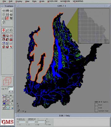
Figure 3. The GMS interface of the groundwater flow model.
Illustrates are the locations of surface water (blue); constant head
boundaries (orange) and cells that are modeled (in black).
We followed Pijanowski et al. (in press) to develop the appropriate driving variable grid representations, which were then converted to a tabular format for input to the neural net software (see below for more details). The neural net trained on the input and output data for 500 cycles, after which no significant reduction in mean square error between the modeled output and presented data was observed. The testing exercise that followed used driving variable input from all cells (except those located in the exclusionary zone) in the study locations but with the output values removed. The network file generated from the training exercise was used to estimate output values for each location. The output was estimated as values from 0.0 (not likely to change) to 1.0 (likely to change); the output file created from this testing exercise is called a "result" file. The actual number of cells undergoing transition during the study period for each county was then used to determine how many cells from each county "result" file should be selected to transition. Cells with values closest to 1.0 were selected as locations most likely to transition. Following Pijanowski et al. (in press), population forecasts were then used to scale the amount of future urban use for the county.
Hydrogeology Model Development
A 3-dimensional groundwater flow model of the GTBW was developed with 100-meter by 100-meter finite difference grid cells using MODFLOW (Macdonald and Harbaugh, 1988). The dimensions of the entire grid were 928x837 corresponding to the grid dimensions of the LTM. The hydrologic model has over 1,000,000 active cells, with more than 34,000 river cells (including lakes). The Groundwater Modeling System (BYU, 1994) preprocessor allowed us to convert GIS-based data into model input files (Figure 3). This ability to incorporate GIS coverages into the model is necessary to examine the influence of land use on groundwater flow and solute transport at these scales. Geological data to parameterize the model was derived from the Michigan Comprehensive Resource Inventory and Environmental System (CRIES) (Schultink et al. 1989) and from county well log data. Details of the model development, calibration and analysis of road salt application are beyond the scope of this paper although details can be found in Boutt et al. (2001).
The following spatial data layers were used in modeling of groundwater flow and solute transport throughout the GTBW:
Surface elevation: surface elevation was developed by merging 30-m DEMs acquired from the USGS. Locations of rivers and shorelines were matched to existing river and shoreline GIS layers from MiRIS.
Bedrock depth: depth to bedrock was quantified by extracting information from over 70,000 well-log points throughout the region. Over 50% of the points were removed from the original database due to likely errors (see Boutt et al., 2001). A depth to bedrock "surface" was developed by kriging these data to the model grid.
Aquifer thickness: the aquifer thickness, including the saturated and unsaturated zones, was created using the GIS by subtracting the surface elevation and depth to bedrock.
Hydraulic Head: the depth to the water table was assessed in the field by measuring the depth to the water table for 22 USGS research wells. This information was converted into water table elevation, which was then used to calibrate the model.
Geologic Properties: The hydrogeologic properties of the aquifer material were quantified by assigning a relative hydraulic conductivity values to a discretized geologic map from CRIES.
Road Salt Application. Locations of roads that have been salted over the last 30 years were acquired from each of the five county road commission offices in GIS format. These layers were then used to apply halite, in reasonable quantities, to the roads. Halite, which is a conservative substance in groundwater, was assumed to be carried into the groundwater system through snowmelt and precipitation.
RESULTS AND DISCUSSION
Land Transformation Model
The results of the LTM simulation for Grand Traverse County are provided in Figure 4. Recall that land use data used for training of the neural network were from the 1980 and 1990 databases. Population forecast data for the county were used to then project out the next locations that were expected to transition to urban (following procedures in Pijanowski et al., in press). Time steps of 2000 and 2020 were then mapped using the GIS.
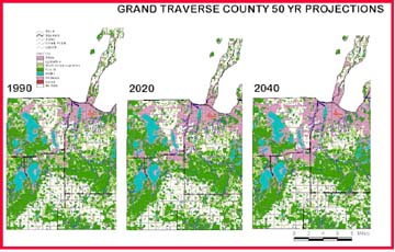
Figure 4. Urban land use projections using the neural net-based LTM,
for Grand Traverse County, Michigan. Urban use is illustrated in pink.
The LTM was used to forecast to 1990 and a change map of the differences between observed and predicted are shown in Figure 5. During the entire model development, these maps were used as visualization tools to discern the types of spatial error patterns that might suggest missing driving variables. A 49% percent correct match of targets and observed urban change was obtained in this final model simulation presented in Figure 5 (correctly modeled targets are in red; locations not correct are in blue).
Future urban development in this county is anticipated along the US 31 highway that runs east-west through the large lakes in the county. In addition, urban development up the Old Mission Peninsula is also p6ssible. Urban development along the northwestern portions of the county, near 3 and 4 Mile Roads, is also anticipated.
A comparison of the model results against historical changes (1980 to 1990) are given in Figure 5. The areas in blue are mostly along two transportation corridors, one extending east-west just north of Lake Anne and the other extends the to south of Boardman Lake. Introducing factors that may be responsible for these urban growth patterns would likely improve the model results.
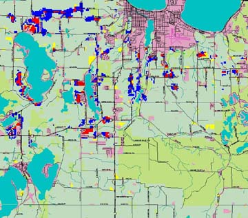
Figure 5. Map comparing locations of LTM predicted and observed
changes in urban use. Locations shown in red are correctly identified
to change to urban by the LTM.
Hydrogeologic Models
Three-dimensional views of the three main aquifer surfaces (bedrock, hydraulic head and glacial drift thickness) are illustrated in Figure 6. ArcView 3D Analyst was used to construct this visualization with each surface exaggerated by a factor of 3.0. Figure 6A shows depth to bedrock throughout the watershed. The bedrock surface of this area is very complex; areas below the Boardman River contain the deepest bedrock surfaces.
Figure 6B shows the depth to the top of the saturated zone of the modeled aquifer. This figure illustrates that the water table is highest in the southeast portion of the watershed. The groundwater elevations for the unconfined aquifer ranged from 375 meters in the very western portion of the watershed to 177 meters along Lake Michigan, Lake Charlevoix, and Grand Traverse Bay (Figure 6B). The thickness of the modeled aquifer is shown in Figure 6C. Thickness varies greatly throughout the watershed; the thickest areas are located in the Pere Marquette State Forest.
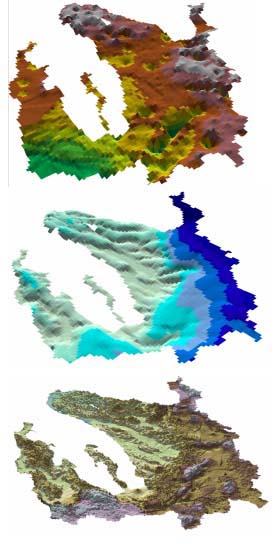
Figure 6. Hydrogeologic data used to parameterize the groundwater
and solute transport models. Data shown are A) depth to bedrock B)
depth to water table and C) glacial drift thickness (thickness of the
modeled aquifer)
A comparison of hydraulic head obtained from the field at the twenty-two USGS monitoring wells with model predicted hydraulic head at those locations was highly correlated, reflecting that that model predicts hydraulic head very well (see Boutt et al., 2001).
A screen grab of the groundwater flow model (Figure 7) illustrates the potential impact of groundwater on stream recharge in two creeks of the watershed located along East Grand Traverse Bay. The blue arrows indicate the relative amount of water entering the streams from groundwater. As much as 90% of the water volume during baseflow of a stream is derived from groundwater (Hyndman, unpub). This graphic also illustrates the importance of how small changes in a land use change location may affect one stream over another.
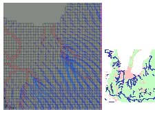
Figure 7. Screen grab of the groundwater flow model.
Stream nodes are illustrated with red; blue arrows
indicated the flow streams. Cell size is 100m x 100m.
Location of the zoomed in area is shown on the right
with a red box.
Figure 8 shows the results of the solute transport modeling simulation using chloride as the tracer substance. This illustration shows that halite application on roads can have a considerable temporal impact across this watershed; even after a fifty-year simulation, chloride only travels 40-50 miles. In some cases, the temporal legacy of land use in this watershed will exceed 100 years.
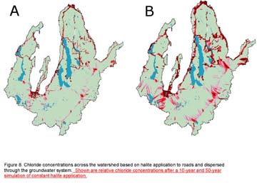
Figure 8. Chloride concentrations across the watershed based on halite
application to roads and dispersed through the groundwater system.
Shown are relative chloride concentrations after a 10-year and 50-year
simulation of constant halite application.
CONCLUSIONS
In this paper, we showed how we used a GIS and Artificial Neural Network based Land Transformation Model (LTM) to forecast urban uses into the future. Anticipated urban uses appear to occur in several important areas in Grand Traverse County. North of Lake Anne, along the US 31 corridor and in the northwestern portion of the county.
A coupled groundwater flow and solute transport model was used to illustrate the relationship between land use and groundwater dynamics in this watershed. We showed that land use derived solutes that permeate the groundwater system can have a long-term affect on water quality. We term this temporal lag effect of land use impacts on the groundwater system, "land use legacy".
Finally, because all three models are tightly coupled to GIS, the large number of cells that are modeled here (over 1,000,000) make management of data for model input and output relatively easy. In addition, GIS is an excellent visualization tool allowing researchers to communicate the results of complex models in an effective and efficient format.
References
Boutt, D.F., D.W. Hyndman, B.C. Pijanowski, and D.T. Long. 2001. Identifying Potential Land Use-derived Solute Sources to Stream Baseflow Using Ground Water Models and GIS. Ground Water 39 (1): 24-34.
BYU, Brigham Young University. 1994. D.O.D. Ground Water Modeling System (GMS), Salt Lake City, UT.
Corwin, DL., Vaughan P.J., and Loague K. 1997. Modeling nonpoint source pollutants in the vadose zone with GIS. Environ. Sci. Technol. 31:2157-2162.
Doe, W.M., Saghafian, B., and Pierre, Y.J. 1996. Land-use impact on watershed response: the integration of two-dimensional hydrological modeling and geographical information systems. Hydro. Proc. 10: 1503-1511
Field, C.K., Sover, P.A., and Lott, A. 1996. estimating the effects of changing land use patterns on Connecticut Lakes. J. Env. Qual. 25: 325-333
Flintrop, C.B., Hohlmann, T., Jasper, C., Korte, O., Podlaha, S., Scheele, S. and Viezer J., (1996) Anatomy of pollution: streams of North Rhine-Wesphalia, Germany, American Journal of Science 296: 58-98.
Fraser R.H., Barten, P.K., and Pinney D.A. 1998. Predicting Stream pathogen loading from livestock using a geographical information system-based delivery model. J. Environ. Qual.: 27:935-945
Herlihy, A.T., Stoddard, J.L., Johnson, C.B., 1998. The relationship between stream chemistry and watershed land cover data in the Mid-Atlantic Region, U.S. Water, Air, Soil Poll. 105:377-386.
Hunter C., McDonald, A., and Beven, K. 1992. Input of fecal coliform bacteria to an upland stream channel in the Yorkshire Dales. Water Res. Research 28: 1869-1876.
McDonald, M.G. and A.H. Harbaugh. 1988. A modular three-dimensional finite-difference ground water flow model. In techniques of water-resources investigations of the United States Geological Survey, Book 6, Chapter A1.
Pijanowski, B.C., D. Brown, B. Shellito and G. Manik. In press. Using neural networks and GIS to forecast land use changes: A Land Transformation Model. Computers, Environment and Urban Systems.
Pijanowski, B.C., S.H. Gage, D.T. Long & W. C. Cooper. 2000. A Land Transformation Model: Integrating Policy, Socioeconomics and Environmental Drivers using a Geographic Information System; In Landscape Ecology: A Top Down Approach, Larry Harris and James Sanderson eds.
Pijanowski, B.C., T. Machemer, S.H. Gage, D. T. Long, W. E. Cooper and T. Edens. 1996. The GIS syntax of a spatial-temporal land use change model. In Proceedings of the Third Conference on GIS and Environmental Modeling. GIS World Publishers - CD-ROM.
Rumelhart, D, Hinton, G & Williams, R. 1986. Learning internal representations by error propagation. Parallel Distributed Processing: Explorations in the Microstructures of Cognition, 1 edited by D.E Rumelhart and J. L. McClelland (Cambridge: MIT Press), pp. 318-362.
Schultink, G., S. Nair, W. Enslin, B. Buckley, J. Chen, D. Brown, S. Chen and B. Parks. 1989. User’s Guide to the CRIES Geographic Information System, Version 6.2, CRIES, RDOP-CRIES-89-2, Michigan State University.
Scott, C.A., Walter, M.F., Brooks, E.S., Boll, J., Hes, M.B., and Merrill, M.D. 1998 Impacts of historical changes in land use and dairy herds on water quality in the Catskills Mountains. J. Environ. Qual. 27:1410-1417.
Skapura, D., 1996. Building neural networks. New York: ACM press.
Skop, E. and Sorensen, P.B. (1998) GIS-based modeling of solute fluxes at eh catchment scale: a case study of the agricultural conribution to the riverine nitrogen laosing in the Vejl Fjord catchement, Denmark. Eco. Mod. 106:291-310.
Swingler, K. 1996. Applying Neural Networks: A Practical Guide. Morgan Kaufman Publishers, San Francisco, California. 303 pp.
Thorburn, P.J., Cowie, B.A., and Lawrence, P.A., (1991) Effect of land development on groundwater recharge determined from non-steady chloride profiles. J. Hydro. 124:43-58
Vesterby, M., & Heimlich R., 1991. Land use and demographic change: results from fast-growing counties. Land Economics, 67(3), 279-291.
Weiskel, P.K., Howes, B.L., and Heufelder, G.R. (1996) Coliform contamination of coastal embayments: sources and transport pathways. Envi. Sci. Tech. 30:1872-1881.
Wiley, MJ, Kohler, S.L., and Seelbach P.W. (1997) Reconciling landscape and local views of aquatic communities: lessons from Michigan streams. Freshwater Biol. 37:133-148.
Zell, A., Mamier, G., Vogt, M., Mache, N., Hübner, R., Döring, S., Herrmann, K., Soyez, T., Schmalzl, M., Sommer, T., Hatzigeorgiou, A., Posselt, D., Schreiner, T., Kett, B., & Clemente, G. 1996. Stuttgart Neural Network Simulator v4.2. [ftp.informatik.uni-stuttgart.de in /pub/SNNS/SNNSv4.1.tar.Z]. Stuttgart: Institute for Parallel and Distributed High Performance Systems, University of Stuttgart.
Author and Copyright Information
Copyright 2001 by Author
|